
Titanic: Machine Learning from Disaster
Explore how to predict survival on the Titanic using machine learning techniques like Random Forest and Logistic Regression. Learn about feature engineering, model evaluation, and implementation examples in Python.
You’ve probably heard the story — or seen the movie. The Titanic was one of the most infamous maritime disasters in history, claiming over 1,500 lives when it sank in 1912.
In this project, we’ll use a curated subset of real Titanic passenger data to answer a critical question:
“What sorts of people were more likely to survive?”
Originally, there were over 2,200 passengers aboard the Titanic. The dataset we’ll be working with includes:
- 891 passengers in the training set (used to build and fit our models)
- 417 passengers in the test set (used to evaluate our models)
While this data has been cleaned and simplified to make it easier to work with, it still reflects real individuals and outcomes — providing a meaningful example of how machine learning can be applied to real-world human events.
Before jumping into feature engineering and modeling, it’s good practice to look for a data dictionary. This helps you understand what each variable means and how it might relate to survival. Thankfully, one is provided here:
Data Dictionary
| Variable | Definition | Key |
|---|---|---|
| survival | Survival | 0 = No, 1 = Yes |
| pclass | Ticket class | 1 = 1st, 2 = 2nd, 3 = 3rd |
| sex | Sex | |
| age | Age in years | Fractional if less than 1. xx.5 if estimated |
| sibsp | # of siblings/spouses aboard | |
| parch | # of parents/children aboard | |
| ticket | Ticket number | |
| fare | Passenger fare | |
| cabin | Cabin number | |
| embarked | Port of Embarkation | C = Cherbourg, Q = Queenstown, S = Southampton |
Notes
pclass: A proxy for socio-economic status (SES):
1st = Upper, 2nd = Middle, 3rd = Lowersibsp:
Sibling = brother, sister, stepbrother, stepsister
Spouse = husband, wife (mistresses and fiancés ignored)parch:
Parent = mother, father
Child = daughter, son, stepdaughter, stepson
(Some children traveled only with a nanny — thereforeparch = 0for them.)
Step 1: Importing Libraries
These are the core libraries we’ll use for modeling, visualization, and data wrangling.
from sklearn.metrics import classification_report, accuracy_score
from sklearn.ensemble import RandomForestClassifier
from sklearn.linear_model import LogisticRegression
import re
import pandas as pd
import numpy as np
import matplotlib.pyplot as plt
Step 2: Load and Prepare the Training Data
We’ll load the training dataset directly from GitHub. We also one-hot encode the Sex and Embarked columns for modeling later.
train = pd.read_csv('https://raw.githubusercontent.com/towardsuffering/data/refs/heads/main/train.csv')

# Encode categorical variables
sex = pd.get_dummies(train.Sex, prefix='Sex').iloc[:, 1:]
embarked = pd.get_dummies(train.Embarked, prefix='Embarked')
train = pd.concat([train, sex, embarked], axis=1)
Step 3: Feature Engineering
We’ll extract titles from names and bucket ages into decade groups. This provides useful context and reduces noise in modeling.
def get_sirname(name):
    if re.search(r'\b(mr|master|rev)\b', name, re.I):
        return 1
    elif re.search(r'\b(miss|ms)\b', name, re.I):
        return 2
    elif re.search(r'\b(mrs|jr)\b', name, re.I):
        return 3
    else:
        return 0

train['age_group'] = train['Age'].apply(lambda x: 0 if np.isnan(x) else int(int(x - 1)/10) + 1)
train['sirname'] = train['Name'].apply(get_sirname, 1)
Step 4: Train the Random Forest Classifier
We train a basic Random Forest using engineered features and visualize feature importance.
features = ['Pclass', 'Parch', 'Embarked_C', 'Embarked_Q', 'Sex_male', 'age_group', 'sirname']
clf = RandomForestClassifier()
clf.fit(train[features], train['Survived'])

importances = clf.feature_importances_
sorted_idx = np.argsort(importances)
padding = np.arange(len(features)) + 0.5

plt.barh(padding, importances[sorted_idx], align='center')
plt.yticks(padding, np.array(features)[sorted_idx])
plt.xlabel("Relative Importance")
plt.title("Variable Importance")
plt.show()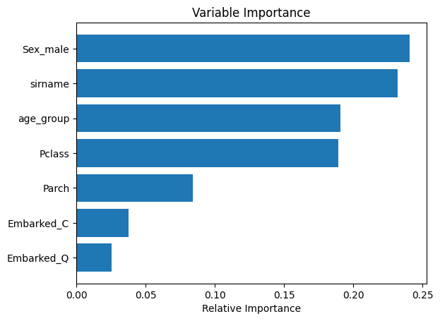
Step 5: Evaluate on Training Data
We evaluate the model using accuracy and classification metrics.
X = train[features]
Y = train['Survived']
Y_pred = clf.predict(X)

print('Correctly predicted on TRAINING SET: {}, errors:{}'.format(sum(Y == Y_pred), sum(Y != Y_pred)))
print(classification_report(Y, Y_pred))
print('Accuracy on TRAINING set: {:.2f}'.format(accuracy_score(Y, Y_pred)))
Step 6: Test Set Predictions
We prepare the test set using the same feature pipeline and generate predictions.
test = pd.read_csv('https://raw.githubusercontent.com/towardsuffering/data/refs/heads/main/test.csv')
sex = pd.get_dummies(test.Sex, prefix='Sex').iloc[:, 1:]
embarked = pd.get_dummies(test.Embarked, prefix='Embarked')
test = pd.concat([test, sex, embarked], axis=1)

test['age_group'] = test['Age'].apply(lambda x: 0 if np.isnan(x) else int(int(x - 1)/10) + 1)
test['sirname'] = test['Name'].apply(get_sirname, 1)

X_new = test[features]
new_pred_class = clf.predict(X_new)

pd.DataFrame({'PassengerId': test.PassengerId, 'Survived': new_pred_class}).set_index('PassengerId').to_csv('decisionTree.csv')
Step 7: Logistic Regression Model
We train and evaluate a logistic regression model for comparison.
logreg = LogisticRegression()
logreg.fit(X, Y)
Y_pred = logreg.predict(X)

print('Correctly predicted on TRAINING SET: {}, errors:{}'.format(sum(Y == Y_pred), sum(Y != Y_pred)))
print(classification_report(Y, Y_pred))
print('Accuracy on TRAINING set: {:.2f}'.format(accuracy_score(Y, Y_pred)))
Conclusion
We’ve walked through building and evaluating two models to predict survival on the Titanic dataset. While Random Forest provides flexibility and feature importance, Logistic Regression gives us an interpretable baseline. This workflow is a strong foundation for real-world classification problems.